Medellín geovisor: a guide to maps, planning and statistics

GeoMedellín, Mapas Medellín and the GeoSAT geovisor

A geovisor is an application for exploring geographic information on a map. GeoSAT’s Medellín geovisor lets you explore neighborhoods, planning layers, population and other public sources; open records, create thematic maps and analyze loaded data. It runs in your browser, free and without an account.

If you arrived searching for “Medellín Geo” or “GeoMedellín”, it helps to distinguish the tools. GeoMedellín is the District’s official geographic portal, bringing together applications, open data, geoservices and documentation. It links to Mapas Medellín, the geographic catalog and the imagery bank. GeoSAT develops this independent geovisor to explore and analyze selected public sources. It is not the City government’s portal.

The District’s description of its GeoMedellín portal ↗

This guide covers the tools available in GeoSAT. To choose a layer and check its date and publisher, read the catalog before starting an analysis. View integrated data →

Find a place

Search accepts neighborhood names, places, addresses and coordinates. It helps you navigate; it does not certify an address or parcel boundary.

1. Type a name in Explore, such as Museo de Antioquia or Parque Iglesia San Agustín. The index searches neighborhoods, heritage, public space, cycling corridors, EnCicla points, tourist attractions, libraries and bicycle parking addresses without sending the text to another service. Use arrow keys and Enter or select a match; a catalog record enables its layer and opens its details.
2. Check the layer below each result: one place may have several representations. The location is a reference center, not an entrance. For another address, use Search addresses with Photon, even when local matches already exist.
3. To reach a known point, enter latitude and longitude in decimal degrees, separated by a comma: 6.2442, -75.5812. Check that the point is within Medellín.
4. Use + and − to change scale. View whole city restores the municipal extent. My location requires browser permission.

Submitted Photon searches pass through GeoSAT’s function. Avoid unnecessary personal information. Search text and precise coordinates are excluded from analytics.

Choose what appears on the map

A layer represents a set of features: neighborhoods, facilities, planning polygons or buildings. Explorations groups related layers and opens tools to explore them. Layers lets you manage each dataset individually.

1. In the Explorations list, check a topic to add its layers without leaving the list. Wait for them to load; some require a closer zoom before geometry is downloaded.
2. Check other topics to combine them. For example, Neighborhoods and districts alongside Public transport routes puts published itineraries in their boundary context. Use the search icon beside Explorations to find a topic.
3. Select an exploration name or arrow to open its tool, such as routes, rainfall or sport, or its Results. If it is not checked yet, it is also added to the map. Use Explorations to return to the same list; other topics remain selected.
4. Uncheck a topic to remove that exploration. Manual layers remain; a shared layer stays while another selected exploration needs it.
5. Open Layers to hide or show a layer without removing it. You can also add individual layers or upload your own files there. Sources and dates and User guide stay at the foot of the panel; the guide opens in another tab.
6. Under Layers, open a layer’s settings to adjust opacity, order or color. Reduce polygon opacity when you need to read the basemap.
7. Switch between Night, Paper and Orthophoto using the map controls. Municipal imagery contains different acquisition dates.

The viewer supports up to eight selected explorations and eight public layers. An exploration can use several layers; if another will not fit, remove an exploration or a layer before adding it. Each response contains up to 500 features and 2 MB per layer. Reference publications load matching pages automatically: the counter shows how many features in the area have arrived. Wait for loading to finish before interpreting statistics; interrupted results stay marked as partial. Small city-wide layers, such as population and IMCV, stay complete as the map moves. Larger layers follow the view. Reference publications retain their original retrieval date. A partial-result warning means you are not seeing the complete inventory.

Review every identified feature

One click can find several overlapping features. The information panel lets you review them without losing the query location.

1. Click a visible feature to open Feature details.
2. Use the layer selector to narrow the review and the previous and next arrows to move between records. The counter shows your position.
3. Read attributes, source and date. Focus this feature fits the map to the selected geometry.
4. To inspect features without pointing at the map, open Add layers → Results. These lists are also paginated. Filters match an exact field value.

The selection retains features loaded at the time of the click. Pending, failed or partial layers can make it incomplete. Left and right arrow keys move between records; Escape closes the information panel.

Find a postal code and compare it with a neighborhood

Postal districts and neighborhoods serve different purposes. View their polygons together to understand which published code covers an area without treating a postal code as an administrative division.

1. In Add layers, enable Postal districts · Medellín and surroundings and Neighborhoods. Wait for the postal publication to finish loading: it contains 59 polygons and requires more than one results page.
2. Locate the address or place of interest. Reduce one layer’s opacity and click the postal polygon to read Postal code and Postal zone. If the location is near a boundary, check both sides.
3. To inspect a known code, open Inspect and export results for the layer and filter Postal code, for example 050011. Keep leading zeros: this is an identifier, not a quantity to average.
4. In Thematic maps, compare codes as categories. In Analyze data, choose a neighborhood as the scope and inspect intersecting postal records; selection does not clip polygons or establish a one-to-one correspondence.
5. Include the code, location and source in your result. When exporting to a spreadsheet, import the column as text so that 050011 does not become 50011.

Synchronization on September 28, 2026 does not establish when boundaries were revised. Polygons include neighboring municipalities. Confirm delivery codes with the relevant operator; the map does not certify deliveries or individual addresses.

Check Medellín planning maps step by step

An initial POT query helps identify the layers and documents to review for a location. Establish the location first, then read each theme separately. One color does not summarize all planning conditions.

1. Search for the address or navigate to the location. Check streets and boundaries; a search point is not a parcel outline.
2. Under Explorations, select Land use and planning and wait for classification, uses and treatments to load. Use Explorations to return to the list and check Neighborhoods and districts for context. Both explorations stay selected. Select a name to open its Results, and zoom in if the query requires it.
3. Click the location and move through layers in Feature details. Note the layer name and published category. If a polygon hides another, reduce opacity or use previous and next to inspect the records.
4. To read the planned structure of the city, add Strategic intervention areas and Urban and rural centers. Compare area, hierarchy or published status; MEDRío and the other areas are planning references, not reports of completed works.
5. For rural land, add Rural agricultural district and Rural planning units. Read the district’s rural-district and treatment code, and each planning unit’s name, classification and category. The 69 district records are not 69 districts; the 22 planning-unit polygons do not establish subsequent adoptions or parcel boundaries.
6. Open Source and scope and follow the official service or document link. These four layers retain December 17, 2014 dates. For numeric parameters, continue with the density, floor-area-ratio and height chapter; for a location’s legal conditions, also verify applicable rules.
7. To study planned gathering spaces, add Proposed public space. Its 480 records belong to the 2014 plan: compare Category, Subcategory or Level in Thematic maps. For example, Mirador Panorámico includes 29 records. Inspect names and dates in their records; polygons do not establish open parks or completed works. Keep this view separate from Parks and public space and do not sum their areas as additional land.
8. Prepare findings and questions to check with the planning authority. Sources and dates and User guide remain available at the foot of the panel. Return to Explorations and uncheck a topic when finished; other explorations and manual layers remain. When the point is near a boundary or a source does not respond, retain that limitation in your notes.

Expected result: an initial reading of published layers and their sources. The viewer does not issue planning determinations, permits, certificates or an automatic conclusion about what can be built. An empty layer does not establish that a restriction is absent.

Map planning density, floor-area ratio and height

To compare development parameters, start with one variable and a concrete question: what maximum housing density does the plan publish for this area? The layer combines 386 municipal urban and urban-expansion polygons with parameters from the 2014 land-use plan.

1. In Add layers, enable Housing density, floor-area ratio and height · 2014 plan. Open Thematic maps and select maximum housing density. The unit is dwellings per hectare, not residents per hectare or existing dwellings.
2. Select a polygon and read its treatment and calculation basis. Density and floor-area ratio use net land area, except Development treatment, which uses gross area. Compare records with a compatible basis.
3. Switch to floor-area ratio to compare permitted floor m² per land m², or height to compare floors. A ratio of 2 expresses an area relationship; it does not mean two floors or independently establish the permitted floor area of a property.
4. Read the published categories alongside the numeric field. N/A and Variable 1/2/3 are not converted to zero; the record retains the text so you can investigate the applicable condition. Do not color missing values as zero development rights.
5. Open Analyze data and inspect the distribution and extreme records. A simple mean describes polygons with values; it is not area-weighted and does not calculate citywide development capacity. Keep variable, unit and classification method consistent when comparing areas.
6. Before using the map in a technical report, open Source and scope and check the articles and conditions of Agreement 48 of 2014. If you compare with Treatments, its 522 metropolitan records have a different scope from these 386 municipal polygons.

Result: a map of published 2014 planning parameters with an interpretable legend. It does not measure actual building heights or replace a planning determination. Density, floor-area-ratio and height services repeat the same records and are integrated once to avoid tripling counts.

Distinguish hazard and risk conditions

Flood, landslide and torrent-flow hazards, risk-management plan scenarios and areas with risk conditions answer different questions. Each layer retains its source, classification and dates.

1. Under Explorations, choose Landslide hazard. The complete 2,376-polygon planning reference loads with the four colors from the official legend.
2. Read the hazard degree: very low, low, medium or high. Select a polygon to inspect Hazard degree, Category, Adoption date and Update date in map service.
3. Open Analyze landslide hazard to compare records by degree. Switch to Flood hazard to inspect its 716 polygons and four degrees separately. Counts describe polygons, not events or affected people; summing polygon areas does not measure population exposure.
4. The Torrent-flow hazard exploration loads 115 polygons: 52 low, 32 medium and 31 high. Read its separate blue legend and choose Analyze torrent-flow hazard to review each degree. Keep its classification separate from flood hazard.
5. The Risk-management plan scenarios exploration loads 507 polygons in three layers: 63 mass-gathering, 409 wildfire and 35 technological-hazard records. Read magnitude in its legend, noting that mass gatherings use Medio and Bajo while the others use Media and Baja; technological hazard keeps six NA records without interpretation.
6. For a different question, enable Risk conditions in Explore. Inspect the type and description in each record without treating the two layers as equivalent.
7. Follow Source and scope to metadata, the official adopted map and the land-use plan. Consult Planning for authoritative decisions about a property.

The plan was adopted under Agreement 48 of 2014. Flood and landslide records state an April 30, 2026 update; torrent-flow records retain April and July 2026 dates; metadata retains a 2016 revision and an earlier count. The 507 risk-management plan scenarios publish no dates. The publication retrieved in September 2026 retains every source ID, with planning geometry adapted by up to one meter for display and risk-management plan geometry left unsimplified. It is not a warning, property assessment or guarantee of stability or safety.

Compare with meaningful colors

Thematic maps sits next to Explore. It represents distinct categories or numeric differences on a layer’s geometries.

1. Enable Population by year and open Thematic maps. Choose the layer and variable to compare.
2. Select Show this map if the style is not yet applied. Use the year control to explore 2018–2030 projections; intervals stay comparable across years for the loaded territories.
3. Open Adjust the map to change colors or grouping. Equal intervals compares magnitudes; quantiles seeks similarly sized groups while keeping tied values together.
4. Select a legend group to highlight its features. Review records opens those features; Show all restores the full comparison.

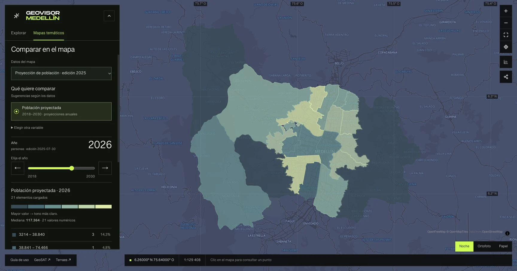
A color does not imply an area is better, worse or dangerous. Read the legend’s variable and unit. Missing values are not zero. Population projections are estimates, not live readings.

Turn the map into an explanation

Analyze data opens the full-screen statistics workspace. You can also enter through the map’s statistics button or Open full analysis in Thematic maps.

1. Choose a layer and variable. Categories allow frequency comparisons; numeric variables show a distribution and summaries such as minimum, median, average and maximum.
2. Explore the visualizations available for that type of data. Annual series show change over time; identifiers should not be interpreted as quantities.
3. Select a category or interval to locate its features and review their records. Return to the analysis to keep the context.
4. For population, open Medellín’s complete statistics: compare all 21 districts, explore the age and sex pyramid and enable the 2018 outline. Percentage compares composition; People compares counts. Download the complete series or share the link with year, district and selection.

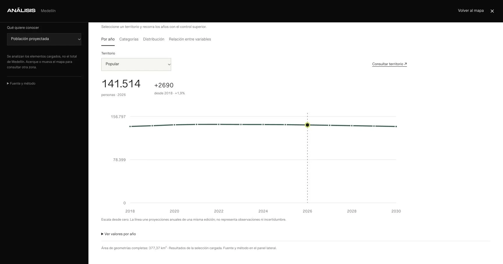
Summaries describe loaded data, not an automatic census of all Medellín. Area sums whole geometries without clipping or dissolving overlaps; it may differ from unique covered area.

For city totals: explore the complete Medellín population series, 2018–2030 →

Choose a chart and interpret the numbers

The chart should answer the question you want to explain. First identify the unit, scope and what one row represents. A row can be a polygon, route segment or inventory component; it is not always a unique entity.

1. To compare types, use categories: each group contains records with a common value. A percentage describes the analyzed selection; check its denominator before generalizing to the city.
2. To understand a numeric variable, inspect its distribution and median. The median is the middle value among valid records; a few extreme values can strongly affect the average. Neither automatically represents a typical resident.
3. To study change, use a time series of the same variable and release. For population, distinguish the estimated year from the year when the projection was published.
4. To explore two numeric variables, inspect the scatterplot when available. A visual association alone does not explain causation: size, coverage or recording practices can influence both variables.
5. To show territorial differences, use a thematic map. Equal intervals keeps numeric widths equal; quantiles divides records into similarly sized groups. Changing the method can change colors without changing any data.
6. Review missing values. An absent value is not zero and should not become a conclusion about the area. Use Records to check a category or extreme value against its record.

Before publishing a comparison: the same variable, the same unit, compatible dates, sufficient coverage and an explicit method. A darker map does not by itself mean greater risk, lower quality or higher priority.

Analyze an area and compare territories

Scope determines which features enter the analysis. Start with a concrete question, such as: which loaded facilities intersect this neighborhood?

1. Enable the layer to analyze and, if needed, a boundary layer such as Neighborhoods and districts.
2. In analysis, change Where to a neighborhood or boundary, a radius around the map center, a drawn area or an intersection with another layer.
3. To draw, place vertices on the map and finish with Analyze area. Undo removes the last point. The boundary cannot cross itself.
4. In the territory comparison, choose Area A and Area B from the same boundary layer and compare the same variable.

Selection uses geometry intersections, including boundary touches. A feature touching two areas can appear in both. Radii are approximate and analysis works on already-loaded features.

Find a bus route and distinguish its directions

Public transport routes brings together 504 municipal paths from August 2025 and queries published stops separately for each itinerary. The explorer organizes the paths into 252 route identifiers so you can find them by name, code or operator.

1. Under Explorations, open Public transport routes. Search Campo Valdés, Floresta, Coonatra or a route code.
2. Compare the name and operator before choosing. One code can refer to several routes: code 107 corresponds to six municipal identifiers.
3. Open a route and choose Origin–destination or Destination–origin. The map highlights the selected path and dims the network for context. Fit route frames its complete geometry. Direction names come from the source; they do not verify that coordinate order follows vehicle travel.
4. In Explore this path, use Play path and Pause path to follow the line. You can also drag Position along path or focus the slider and use the arrow keys. A and B mark geometric endpoints, not terminals or stops.
5. If Part 1 / 2 appears, use Previous part and Next part to explore each part separately; the viewer does not connect gaps. With reduced motion enabled, use the manual slider; playback is disabled.
6. Inspect the operator, type, municipal identifier and record date. Length was calculated on the original geometry before simplifying its display for the browser.
7. Under Published stops, inspect records joined by municipal route identifier and published direction. Search an address or stop-location ID; the list shows twelve records and Show more stops reveals the next set. The number is the source value and may skip or repeat.
8. Open a stop to inspect its address, identifiers and individual date; use Back to route to recover the itinerary. Stop positions remain as published, without snapping to the path. An empty list can mean that this direction has no associated records; it does not prove that the service has no stops.
9. Open Thematic maps or Analyze data. Select this layer and Type or Published operator to compare the loaded paths. Statistics count paths: both directions of one route are two records.

Paths are an August 14, 2025 reference. The stop inventory queried on September 28, 2026 links 10,043 rows to 247 of 252 routes and 493 of 504 directions; the same stop can occur on several routes. Record dates run from 2018 through February 2026, and 6,882 rows retain a 2018 date. Published numbering and point position do not establish a navigable sequence or exact path alignment; there is no geometric snapping. No timetables, arrivals, frequencies, fares, traffic, verified accessibility or live vehicles are provided. Confirm the route and stop with the operator before travelling.

Follow a route and locate its stops

Feeder routes organizes Metro’s published mapping for service areas 3 and 6. It groups itineraries by route code so you can distinguish individual paths.

1. Under Explorations, select Feeder routes. Search by code, such as C3-004P, or destination, such as Belén.
2. Open a route and choose its itinerary or direction. The map highlights that path and dims the rest of the network. The published direction does not verify the geometry’s drawing order.
3. Use Explore this path to play or pause the line, or explore it manually with the slider and arrow keys. A and B are geometric endpoints, not terminals. If there are several parts, switch between them with the part buttons; each is explored separately. Reduced motion keeps only the manual control available.
4. Review published stops for the selected itinerary. Select one to center it and open its record.
5. Use Fit route to recover the complete view or All routes to return to the catalog. Follow the operator link before travelling.

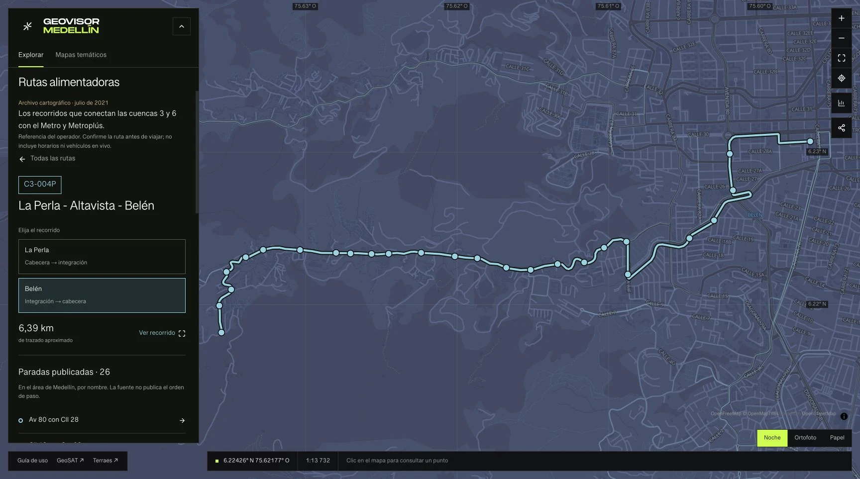
This is reference mapping with July 2021 metadata. It does not establish current operation, frequency, timetables, traffic or vehicle positions. Stops appear by name because the source does not publish their sequence.

Explore the city by bicycle

By bicycle brings together the cycling network and bicycle parking published by Movilidad Humana. Use it to study recorded infrastructure and differences between districts.

1. Under Explorations, choose By bicycle. Lines represent network segments and points represent bicycle parking.
2. Open Thematic maps, select Cycling network and compare Cycling infrastructure type to distinguish shared streets, sidewalk cycleways and roadway cycleways.
3. Select a segment to inspect its name, published length, status and construction year. In Analyze data, compare infrastructure types and review their records.
4. EnCicla stations overlays the metropolitan inventory on the cycling network. Search for Ruta N or Universidad Nacional, inspect its record and use Thematic maps to compare type or Inventory status. Activo, Inactivo and Futuras do not indicate current operation. An unclassified point is retained as a missing value.
5. Select Bicycle parking to compare Recorded parking modules or review records by district. Check the address and record date before planning a visit.

The network and parking are 2025 references. EnCicla does not declare a data date; its item was modified in 2023. All 119 metropolitan points are retained, including records outside Medellín and an unclassified device. Modules are infrastructure, not free spaces. There is no bicycle availability, traffic feed or safe-route calculation. Published length describes each whole segment even when analyzing part of the city.

Read Metro, buses, road infrastructure and walking references

Start with the question: recognize a line or route, locate a stop or taxi stand, or understand a published structure. These layers combine inventories and planning from different periods; they are not a journey planner or a live traffic map.

1. To recognize the published network, enable Mass-transit lines and Mass-transit stations in Add layers. Compare Transport type or Line in Thematic maps and select a station to inspect its name. The 14 paths and 81 station records include neighboring municipalities and records by line; they are not 81 unique Medellín stations.
2. Check Inventory status before presenting a line as operational. Existing, proposed, under construction and under study are source categories with no declared review date. The map does not establish transfers, travel direction, frequency or accessibility; confirm the journey with the operator.
3. In Public transport routes, choose one of the 504 paths and its published direction. The viewer queries stops by exact route identifier and then separates records by direction: matches exist for 247 of 252 routes and 493 of 504 paths. Search the list by address or stop-location ID, use Show more stops to see the next twelve records and open one; Back to route restores the itinerary. Dates belong to individual stops, from 2018 through February 2026; neither published numbering nor point position defines a navigable sequence or an exact fit to the path.
4. To locate a taxi stand, enable Taxi stands and filter District in Inspect and export results. Open one of the 192 records and read its address, number, administrative instrument and published validity year: 2025. In Thematic maps, Published capacity (vehicles) compares capacities from 2 to 29 vehicles; it does not count waiting taxis or free spaces.
5. To inspect a crossing, add Traffic-light crossings. Its 724 records identify crossings, not signal heads or currently working lights. Read the code and address; the map provides no signal cycles, phases, faults or congestion.
6. In Crossing structures and bridges, compare Crossing-structure type. The inventory distinguishes 608 pedestrian bridges, 474 road bridges and 911 buried conduits. Read the address and obstacle crossed before assuming each record is a pedestrian crossing. Anomalous dates and years remain in the record and do not establish age or structural condition.
7. To explore walking interventions, combine Tactical urbanism with Reference pedestrian network · 2014 plan. Compare their statuses separately: the 120-intervention inventory retains an unverified 2028 year, while the 1,314 pedestrian segments belong to the 2014 plan and can extend beyond the district.
8. Add Sidewalks · municipal inventory and zoom to street level (zoom 17). The service contains 42,965 traces, but each query returns up to 500 in the visible area and may be partial. Inspect element and segment codes; do not infer continuity, walking direction or accessibility from the geometry. The source declares no update date or verifiable units for width, height and length, which are not shown.
9. For a planning query, add Road hierarchy or Rural road-corridor reserves. The 1,030 paths and four polygons retain their December 17, 2014 reference. Compare Road hierarchy and Status and read reserve names; a planned widening or reserved corridor does not establish completed construction.
10. In Analyze data, choose an area and inspect the records behind each category. Lines and polygons retain their full geometries: lengths and areas are not clipped to the selected boundary or converted into unique infrastructure. Export with the query theme, date and scope.

Wait for paged loading to finish before counting. The 10,043 stop rows are not 10,043 unique stop locations: one place can occur on several routes, and 6,882 rows retain a 2018 date. Use these layers to research and prepare checks with the relevant authorities. They do not certify traversable routes, continuous sidewalks, reduced-mobility access, bridge safety, current administrative validity or transport availability.

Read SIATA air quality observations

Air quality shows SIATA’s population-representative PM2.5 stations inside the map extent. It includes stations in Medellín and neighboring municipalities; each point has its own value, classification and date.

1. Under Explorations, open Air quality. The panel loads the stations and colors points using SIATA’s published classification.
2. Read the number beside µg/m³ as the mean concentration over the last 24 hours. It is neither an instantaneous reading nor a numerical ICA index value.
3. Select a station to locate it and open its record. Check the source update, expressed in Colombia time (UTC−5), and the station type.
4. Filter the list by Published classification or choose Highest concentration. This organizes the list; it does not extrapolate values to neighborhoods or remove map points.
5. Open Compare readings and inspect data to examine the distribution, review records and export the query with provenance. Concentrations are not summed, and a mean across stations does not represent all of Medellín.
6. Keep the layer visible to check for updates every five minutes. Points turn gray when source updates are older than 30 minutes. If the source fails, the previous query is retained with a notice and can be retried.

Provisional operational data subject to SIATA/AMVA validation. The time belongs to the source publication and does not guarantee the time of the latest measurement. GeoSAT applies the 30-minute freshness criterion; it is not a health category. Custom thematic maps in analysis use exploratory groups, distinct from the official classification. Consult SIATA for recommendations and alerts.

Compare accumulated rainfall by station

SIATA’s rain gauge network shows how much rain has fallen at specific locations in Medellín and its surroundings. Each station publishes accumulations for seven time windows with its own update time.

1. Under Explorations, open Rainfall by station. The map starts with the last hour and lists the largest accumulations with recent updates first.
2. Change Map period to examine five minutes, thirty minutes, one hour, three hours, twenty-four hours, three days or thirty days. Colors and the list change together. The millimeter scale stays fixed so the same color retains its meaning.
3. Find a station by name and select its row to locate it. Use Previous and Next to review the list in pages. Search and sorting organize the list without removing stations from the map.
4. In the record, check Accumulated through, expressed in Colombia time. Zero means the station published an accumulation of zero millimeters. A dash means the value is missing. Gray marks an old update or an unverifiable reading.
5. Under How it has rained, choose a window from 3 hours to 30 days, a gauge and the interval or accumulated series. Browse the curve, expand it and download the CSV with its dates and source. The two gauges are independent instruments: they are neither summed nor averaged.
6. Open Compare accumulations and inspect data to see the distribution for the selected period, compare stations within an area or inspect and export records. The mean describes stations, not average precipitation across Medellín.
7. Share the view to preserve layers, framing and the selected period. Readings are queried again when the link opens; the link does not freeze weather conditions.

Windows end at each station’s published time. They overlap and must not be summed. Millimeters at different stations must not be summed either. Operational data is subject to SIATA validation; it is not a forecast, radar, intensity in mm/h or an emergency alert. Queries refresh every five minutes while the layer and browser tab are visible. GeoSAT marks source updates older than thirty minutes as old.

Compare temperature, humidity, wind and pressure

SIATA weather stations show how observations vary between locations in Medellín and its surroundings. The map starts with temperature and offers four variables with explicit units.

1. Under Explorations, open Temperature, humidity and wind. Choose one of the four Map variable options: point colors and the value in each row change together without another download.
2. Read the legend. Intervals stay fixed for each variable when panning or searching for a station. Temperature is in °C, relative humidity in %, wind speed in km/h and pressure in hPa.
3. Open Find and sort stations to locate a name or compare recent values from highest to lowest or lowest to highest. Old and missing readings follow recent ones. Previous and Next page through the list; searching does not hide map points.
4. Select a station to inspect its record and all variables. Updates appear in Colombia time. A dash means no valid value: zero wind is valid, while zero pressure is discarded.
5. In How it has changed, choose one, three or six hours. Expand opens the series in a full window; Escape returns to the record without losing the selected observation. The curve uses records published every minute for one hour and every five minutes for three or six hours. Changing the variable also changes the map. Hover, tap the curve or use Browse records with the arrow keys to read each observation.
6. Check dates and breaks in the curve: missing values are not filled in. The vertical scale fits the series and the mean uses only valid published records. View records and download opens the table and exports a CSV with UTC dates, units and source. This download covers one station and variable.
7. Open Compare stations and inspect data. Analysis starts with the variable chosen on the map. Explore its distribution, compare an area and inspect dates in the table before exporting. Temperatures, humidity, speeds and pressures are not summed.
8. Share the view to preserve the variable, layers and framing. Reopening it queries available observations; the link does not preserve a historical weather snapshot.

Dates are published station updates. This SIATA service does not declare each variable’s aggregation window. Operational observations are subject to validation. Queries refresh every five minutes while the layer and browser tab are visible. Gray means an update older than thirty minutes, no verifiable value or date, or a failed query. GeoSAT’s scales are not alerts or forecasts. Pressure depends on altitude and is not corrected to sea level; a station mean is not citywide weather.

Browse river and stream water levels

SIATA’s network lets you follow a station over time and relate readings to its channel cross-section when published.

1. Under Explorations, open River and stream levels. Search by name or municipality and select a station to locate it.
2. In Water level and channel profile, choose three hours, twenty-four hours, three days or thirty days. Each period retains its own dates and resolution: one minute, thirty minutes or four hours.
3. Expand opens the curve and profile in a full window. Browse records with the pointer, a tap or keyboard arrows. The selected reading moves the water in the profile; it is not a flood animation.
4. Check gaps and the latest record date. View records and download opens the table and exports CSV with levels in meters, UTC dates, resolution and source.
5. Close with Escape to return to the same station and reading. Consult SIATA for operational information and official alerts.

Level uses each sensor’s local reference, not elevation above sea level or flow. Do not sum stations or interpret a higher level as greater risk. The profile has no declared survey date and its axes use independent scales. Zero and negative values remain missing; they do not prove the channel is dry. Longer windows may omit brief peaks.

Follow the river and streams

Waterway mapping combines 817 drainage records, one Medellín River polygon and 113 wetland and lagoon polygons. Five have published names; 108 do not. Explore the territory and compare published categories; every record reports an update of December 17, 2014.

1. Under Explorations, enable River and streams. The network loads in pages; wait for all 817 records. The river and 113 wetland polygons can be hidden or reordered independently.
2. Search for a stream, such as Q. La Iguaná. For a wetland, open Inspect and export results on Wetlands and lagoons and filter Name, for example Lago del Jardín Botánico. A place may also appear in Water bodies, the earlier layer of five named places: these are not additional sites.
3. On the Drainage network card, choose Compare main and secondary drainage. The legend distinguishes 12 main records from 805 secondary records. Select a group and use Review to browse its records.
4. Open Layer statistics to compare hierarchy or Mapped record length (m). Length is calculated from the entire original geometry in EPSG:9377 before simplification; it is not clipped to the visible area. A drawn analysis area selects intersecting records without clipping their lengths.
5. Add Water-supply catchments · 2014 land-use plan to study 27 planning polygons. Read the name, published water system, rural district and protection category; five records lack a water-system value and two lack a rural-district value. A polygon does not establish current abstraction or operation, or a hydraulic connection to an intake.
6. On Wetlands and lagoons, open Analyze data and inspect Original geometry area (m²). The 113 polygons retain their complete geometries; area describes their mapped footprint. If you choose Name, the analysis separates five published values from 108 unnamed records; a missing name does not mean zero area.
7. For operational readings, open River and stream levels. Choose a SIATA station and inspect its timestamp, curve and channel profile. Share the thematic map or export records from Results with their source and date.

Lines are simplified by up to one meter for display. They do not represent regulated setbacks, flow, water quality or flooded areas. The 817 records are not unique streams. The 113 polygons are not a current field-verified wetland census either: they include the five named water bodies and must not be added to that layer. Their area does not measure water volume or ecological condition; their metadata was revised on March 19, 2015. Catalog and download dates do not change the service’s 2014 date. Water-supply catchments are 2014 land-use-plan reference areas; they do not certify flow, drinking safety or current supply. This dataset is not presented as the municipality’s 2025 satellite model.

Compare historical water campaigns in San Antonio de Prado

The 75 sampling sites and 74 stream-setback quality polygons support research into published assessments of this area. First distinguish what was assessed: a water category and a setback category are different variables.

1. In Add layers, enable Sampling sites · San Antonio de Prado and Stream setback quality · historical. Locate the rural district and select a site to read its name, sector and location.
2. Open Thematic maps and compare the sites’ 2017 campaign category. For other campaigns, select the corresponding field and read its year and variant. Source fields v1, v2 and v3 are not presented as equivalent samples.
3. Select the same site and inspect its 2013, 2015 and 2017 categories in the record. A site date can extend to January 2018 without turning its 2017 category into a 2018 measurement.
4. Switch to the setback layer to inspect IIR categories for 2012, 2013, 2015 and 2017 and published pressures. Keep the layers separate: spatial coincidence does not establish that a sampling site corresponds exactly to a polygon.
5. For territorial context distinct from water quality, enable Water-supply catchments · 2014 land-use plan. Its 27 polygons publish planning areas, not sampling results. Read the name, water system and protection category; five records lack a published water system and two lack a rural district.
6. In Analyze data, compare categories from one campaign and inspect missing information. N/A, Sin observación and Sin información remain missing information or published categories; they are not good results or measured zeros.

Use titles with location, variable and campaign, such as “Published water categories, San Antonio de Prado, 2017”. These data do not establish drinking safety, current quality or health risk; pressures are historical and polygons do not certify current legal setbacks.

Read water intakes, treatment plants and utility networks

Combine published infrastructure to understand an area’s context: intakes, treatment plants, sanitary coverage, substations and main networks. These layers describe inventories and planning with different dates, not the service a home receives today.

1. Enable the Public utilities layers that answer your question. Start with Water intakes and Sanitary coverage and perimeter; wait for paged loading to finish. Reduce perimeter opacity if it hides the points.
2. Search for an intake by name, such as Acueducto Piedras Blancas. The inventory contains 76 records and can represent one water system through several points. Eight unnamed records remain available on the map and in Results.
3. Add Treatment plants · rural water systems and compare Treatment type or Provider in Thematic maps. Open one of its 36 records to read name, process and territory. Proximity between a plant and an intake does not establish a hydraulic connection.
4. For Sanitary coverage and perimeter, compare Category. The 174 polygons include five EPM and 169 other-entity records; they are planning coverage or potential-coverage pieces, not unique companies or household connections.
5. Add Electrical substations · 2014 land-use plan and inspect name and date. The archive retains 26 polygons in Medellín and neighboring municipalities; 22 intersect the viewer extent. Presence does not estimate power ratings or electrical coverage.
6. To follow published alignments, enable Main utility networks · 2014 land-use plan and zoom in until the layer loads. Compare Utility type to distinguish water, sewerage, gas and energy. Each query receives up to 500 segments from the area; if partial, reduce the area before analyzing.
7. Combine the query with River and streams or draw an area in Analyze data. Review the records behind each category and export the result with source and date. Spatial selection retains full geometries and values of intersecting records.

Intakes: individual updates from 2003–2019, with metadata reviewed in 2020. Plants: no review date declared. Perimeters, substations and networks: December 17, 2014 references. The source network contains 14,629 segments, not all loaded at once. None of these layers certifies connection, feasibility, capacity, drinking safety, continuity or current outages.

Find citizen-service offices and social services

Compare 22 citizen-service offices, 96 social-inclusion records, 32 family-commissioner records and ten Peace and Human Rights offices. Layers retain institutional categories and shared locations.

1. Under Explorations, select Citizen services and assistance. Hide each family separately under Layers or search for an office by name.
2. Select an office to read its published address, service and district. Use Previous and Next when points overlap: one location may host several services.
3. Open Thematic maps, choose Social inclusion and Category, and compare the ten published categories. Select a group to review its records.
4. In Statistics, compare categories or districts and inspect missing values. Counts describe source records, not people receiving assistance, capacity or unique buildings.
5. Use Explorations to return to the list. Check another topic to combine it without leaving the list, or select its name to open its tool. Unchecking an exploration removes the layers it introduced, except those needed by another selected exploration. Manual layers and local files remain.

No update date is published. Confirm opening, hours, requirements and availability with the institution. Commissioner points do not establish jurisdiction for a case.

Locate Wi-Fi sites and check what the map covers

Use the inventory to locate sites published as free Wi-Fi near a place. Its 332 records are reference locations: the map does not detect networks or draw the area reached by a signal.

1. In Add layers, enable Free Wi-Fi sites · municipal inventory. Add Neighborhoods for context if needed and wait for loading to finish.
2. Select a point and read Name, Address and Published territory code. Codes identify territories; they are not quantities to average. Record SN01 has no verified territorial equivalent.
3. Open Analyze data and choose a neighborhood or radius as the scope. Inspect selected sites before describing proximity: distance is straight-line and a point does not necessarily identify an entrance.
4. To compare the published distribution, choose Published territory code in Thematic maps. Two records share coordinates; inspect their names with Previous and Next rather than assuming an error or a single installation.
5. Keep the names and addresses you want to verify. Check access conditions with the venue before travelling.

The source declares no update date. It does not confirm a working connection, speed, capacity, signal coverage or free access today. An area with no published points does not establish a lack of connectivity.

Find enterprise support and employment offices

Prepare an inquiry with an institution using its published locations. Compare 16 CEDEZO enterprise centers and 17 OPE employment-office records while keeping each service in its own layer.

1. In Add layers, enable Enterprise development centers · CEDEZO or Employment offices · OPE to match your question. Start with one layer and add another when comparison is useful.
2. Select a location to read its name, address, district and neighborhood. CEDEZO location references help recognize a site; for OPE, read the published service description.
3. From layer settings, open Inspect and export results and filter District, for example Popular. Inspect records to distinguish offices sharing a location.
4. To study distribution, open Thematic maps or Analyze data and compare districts. Counts represent inventory records, not advice sessions, vacancies, people served or unique buildings.
5. Export the selection with its source when preparing a list of places to confirm. Check opening, requirements and programming directly with the institution.

No update date is declared. CEDEZO and OPE can share premises. Coordinator names, personal phone numbers, vacancies and places are not published. Presence in the inventory does not guarantee current operation.

Compare higher education and vocational training

The inventory contains 248 records: 215 vocational-training records and 33 other higher-education types. It complements the separate school-sites layer.

1. Under Explorations, choose Higher education and training. For schools, use the separate School sites exploration.
2. Search for an institution or select its point. Read type, sector, address and district before comparing records.
3. In Thematic maps, compare Type or Sector. In Statistics, review distribution by district; repeated names and locations do not become unique institutions.
4. Share the public map or export attributed records for further analysis. Confirm programs, accreditation, admissions and operation with the institution.

The source declares no update date; 248 records are not 248 universities or unique campuses.

Compare 2024 enrollment, outcomes and school meals

These layers support research into aggregate figures per school site. Each retains 779 records for the published 2024 period; names and locations can repeat. Start with one measure and a specific question, such as how published enrollment varies across sites in one district.

1. In Add layers, enable Enrollment and school outcomes · 2024 records or AM/PM school meals · 2024 records. Wait for both results pages to finish loading before analyzing the collection.
2. Select a site and check Name, Institution, Sector, Service and Reference year. An institution name does not by itself identify a unique site. Compare records where locations coincide.
3. Open Thematic maps and choose Enrolled students to compare quantities per site. The legend represents students in each record, not an enrollment rate, current available places or educational quality.
4. In Analyze data, select a district and inspect the distribution, zeros and extreme records. The outcomes layer retains 58 records with zero enrollment; do not read that value as confirmation that a school closed.
5. Switch to students who passed, failed or dropped out to inspect each count. In the published records, these three quantities sum to enrollment. Do not add them to enrollment again or turn an average count into a rate.
6. For school meals, the measure counts students receiving the AM/PM food strategy within the school. All 303 zeros are retained; the source does not clarify whether each means no beneficiaries or missing reporting.
7. Export the selection with the measure name and Reference year 2024. When comparing areas, keep layer, variable and method consistent and inspect repeated names before claiming a count of unique students.

The layers share sites with the educational inventory and with each other; they do not add new schools. These are 2024 aggregate counts without student names or rates calculated by the viewer. They do not support a quality ranking, causal conclusions or confirmation of current places, menus, eligibility or services. The exact update day is not declared.

Read health facilities as planning records

The 99 polygons belong to the Health Facilities category in the 2014 land-use plan. Use them to read the plan and compare its historical distribution.

1. Open Health facilities in the land-use plan and read the reference date.
2. Select a polygon and inspect its name, neighborhood, level and dates. Some names describe projects, parking or historical providers.
3. Compare Level in Thematic maps, or inspect full areas and categories in Statistics. Do not treat each polygon as a unique institution.
4. When presenting or exporting the map, retain the 2014 planning reference and explain the distinction between a planning facility and a currently accredited service.

This is not a current care directory or an emergency-care locator. It does not establish accreditation, services, opening hours or current access.

Explore recycling and material-recovery stations

The municipal inventory contains 46 ECAS records and 23 organization names across 14 published urban and rural districts.

1. Open Recycling and material recovery. Search for an organization and inspect its acronym, address and neighborhood.
2. Select a point to identify the location. One organization may have several locations.
3. Create a thematic map by district or organization, then use Statistics to inspect each group and its records.
4. Before travelling, check directly with the organization which materials it accepts, its hours and conditions.

The description mentions 45 active ECAS in 2025, while current queries return 46 records. The viewer retains all 46 without asserting current operation or inventing an update date.

Distinguish reserves, protection and ecological structure

A reserve, a protection designation and a planning zone describe different objects. Read them separately before overlaying them: counting polygons or summing their areas does not automatically produce a protected-nature total.

1. Open Reserves and protected areas. Select one of the 17 Guardabosques reserves to inspect name, subcatchment, catchment and rural district. For a designation, also read the published category and document.
2. Create a thematic map by catchment for reserves or by category for designations. Select a group and use Review to browse its polygons and recognize parts sharing a name.
3. Add Environmental zoning · 2014 land-use plan to study how the plan classifies an area. Compare Zoning, Ecological structure or Components and inspect the designation document in the record. Its 207 segments are not 207 distinct protected areas.
4. To inspect planned spatial relationships, enable Ecological connectivity network · 2014 land-use plan and zoom to neighborhood scale. Compare Type or Element and distinguish proposed links and nodes from those classified as current in that plan.
5. Connectivity is queried by area and can return partial results. A planning line or polygon does not establish habitat continuity observed today; keep its date visible when comparing with reserves or forest interventions.
6. Enable Ecoparks · 2024 management inventory to inspect 81 management polygons. Compare Action or Subcategory and read the published name, associated stream and reference address in each record. Compare them with Parks and public space without summing areas: the layers overlap and the 81 records are not 81 new parks.
7. Before exporting areas, read the scope: nine of ten designations intersect the viewer extent; Alto de San Miguel lies to the south. Complete polygons can cross municipal boundaries. Neither summing them nor making a spatial selection automatically clips their area to Medellín.

Reserves and designations: described updates in November and December 2025. Zoning and connectivity: adopted in 2014; “current” and “proposed” are categories in that plan. Designation metadata retains an earlier count of 11, while the queried publication contains ten. Published ecopark management actions do not prove completed works or current access. These do not certify current boundaries, trails or public access; the restoration chapter explains how to read interventions without mistaking them for current forest cover.

Explore forest restoration and seed-source trees

To understand what an environmental project documented, inspect its trees and interventions separately. The inventory includes 89 seed sources surveyed in 2024–2025 and 160 forest-intervention polygons from Más Bosques.

1. In Add layers, enable Seed-source trees and Forest interventions. Add Guardabosques reserves for context if needed, keeping their boundaries visible at low opacity.
2. In Thematic maps, choose seed sources and compare Species. Open a tree to read its survey date, diameter at breast height in centimeters and height in meters. Codes can repeat: each row retains its source identifier.
3. Switch to interventions and compare Catchment or Subcatchment. Read establishment and planting dates before grouping records from different periods; individual dates span 2010–2025.
4. In Analyze data, select a catchment or draw an area and inspect planted trees and published area in hectares. Distinguish that attribute from the area the tool calculates from geometry. Selecting an area includes intersecting records without clipping their values.
5. Open the records behind a category or total and prepare a map with project, period and source. Polygons can represent interventions and maintenance: do not treat their sum as unique hectares of forest without checking overlaps.
6. For a separate inventory, enable Ecoparks · 2024 management inventory and compare Action. Its 81 polygons record 74 Mantenimiento, five Generación and two without a published action. Compare with Parks and public space: the layers overlap and do not represent 81 additional parks or works confirmed today.

Planted-tree quantities are inventory attributes, not survival counts. These layers do not measure current forest cover, captured carbon or restoration success. Precise locations do not establish public access to reserves or trees.

Read rural land cover from the 2021 orthophoto

Use this query to distinguish areas interpreted as forest, pasture, crops or other rural cover. The source contains 19,221 polygons; the viewer receives the nearby area you are viewing, subject to a per-query limit.

1. In Add layers, enable Rural land cover · 2021 orthophoto. Locate a rural area and zoom in until the scale notice disappears; the layer requires zoom 17 or closer.
2. Wait for the response and check whether it is complete. If results are partial, reduce the visible area before comparing categories or areas. Do not treat received records as an entire rural district.
3. Open Thematic maps and compare Land cover (CLC level 3). Names match level-three Corine Land Cover codes checked against IDEAM’s legend; codes without verified equivalents remain explicitly identified.
4. Select a polygon to inspect its class, rural district and published area in hectares. A cover class describes interpretation of the image; it is not a land-use rule or activity permit.
5. In Analyze data, inspect categories and records from the query. Published area describes the entire polygon; selecting a neighborhood, radius or drawn area does not clip that attribute to the selected boundary.
6. Compare with restoration or reserves while keeping their dates and scopes visible. An intervention polygon, a reserve and forest cover can overlap without measuring the same phenomenon.

The reference is 2021 orthophotography, not current cover. Area queries can be partial and do not independently calculate unique forest hectares, deforestation or carbon. Level-four and current-use codes without documented domains are not translated into invented categories.

Explore species in the urban tree inventory

Sistema Árbol Urbano describes species and statuses recorded by the municipality in an area. It includes felled individuals and is not a live census.

1. Under Explorations, open Trees in this area. The map zooms to street scale; move it to the park, street or block you want to inspect.
2. Check the loaded record and species counts. When Partial query appears, zoom in: each query returns up to 500 records and counts do not represent the city total.
3. Open Species map to compare scientific names using colors. Select a legend category and review its records; Other groups the less frequent categories in this query.
4. Use Published status map to distinguish statuses retained by the inventory. Each record separately shows individual status, published condition and update date.
5. Analyze this query opens statistics for the loaded records. Export them from Results. Zooming out suspends the query; Zoom in here enables it again.

Records do not measure canopy cover, shade, carbon capture or tree risk. Do not extrapolate a partial query’s composition to Medellín. Published dates belong to individual records and do not establish a current inspection. Free-text observations and contract and intervention data are excluded.

Find courts, pools and sports facilities

Sport and recreation brings together the 967 records in INDER’s map inventory: 39 facility types, including administrative offices. Use it to locate a place or study how facilities are distributed.

1. Under Explorations, choose Sport and recreation. Wait for the complete publication before interpreting counts.
2. Combine Facility type and Urban or rural district. For example, Piscina and Belén returns three records. Each option shows how many records match the other filter; Clear filters restores the inventory.
3. Choose Fit results to frame them. Open a record from the list and use the arrows to review filtered features. The list has pages of 12; features on other pages remain on the map.
4. Open Analyze to study only the filtered records, or Compare on map to explore their categories. Clear the filters to compare all 39 inventory types. Other groups the less frequent categories and lets you review their records.
5. Share view retains the selected type and district. From the layer settings, Inspect and export results downloads those records. For hours, terms and reservations, follow the link to INDER.

One complex may contain several courts, pools and offices: 967 records are not 967 complexes or available places. The service declares no update date; this publication was retrieved on September 27, 2026. Two records have no published district and remain accessible under that option. Names, categories and territorial labels are retained from the source.

Find places to explore

Medellín’s tourism inventory includes 92 attractions in 32 published categories. Three visitor information points appear in a separate layer.

1. Under Explorations, choose Places to explore. Both complete publications load even when you zoom into a smaller area.
2. Search Parque Explora, Museo de Antioquia or Parque Regional Ecoturístico Arví. Check the result’s layer: a place may also appear in heritage or public space. Select the tourism record to inspect its attributes.
3. Open Inspect and export results from the layer settings. Choose Attraction type, then type or select Museo from the suggestions. Apply the filter to show the nine records in that category. Clear filter restores the complete publication.
4. In Thematic maps, choose Attraction type to compare categories. Other groups the less frequent categories in the query; select it and browse its records to read each place’s original type.
5. Open Analyze data to count by type or district, or choose a radius to study proximity. Distances are straight lines and locations do not identify entrances: confirm access before travelling.

The attractions inventory dates from 2019 with attributes added in 2024; the service and metadata retain different dates from that year. Visitor information points have no declared update date. Neither layer confirms current opening, hours or prices. Website links associated with different places were found during review and are not published. Do not add these records to heritage layers as unique places.

Find libraries and reading spaces

To study, consult a collection or explore cultural facilities, start with Libraries and reading. The map brings together 32 municipal inventory records across urban and rural districts.

1. Under Explorations, choose Libraries and reading. The layer loads all 32 published records so you can compare the whole inventory even after zooming in.
2. Search Biblioteca Pública Piloto, Santa Elena or San Sebastián de Palmitas. Check the result’s layer, then select the library to locate it and open its published name, address, type and territorial classification.
3. In Thematic maps, compare Type to distinguish neighborhood libraries, library parks, the Piloto and its branches, documentation centers, the children’s reading house and historical archive.
4. In Analyze data, compare counts by type or district. Select a category to locate its places and review their records. Archive and documentation-center records do not all represent lending libraries.
5. To study proximity, choose a radius or drawn area. Distance is measured in a straight line: confirm access and services with the institution before travelling.

The 32 records belong to this municipal map service; they are not a census of every Medellín library. The source does not declare an update date or confirm current opening, hours or events. Published territorial classifications are retained.

Read the cultural heritage map

Architects, researchers and visitors can explore heritage published by Planning while keeping cultural valuation and legal designation distinct.

1. Under Explorations, choose Cultural heritage. The map opens central Medellín with designated cultural assets (BIC), valued-heritage points and influence zones. Each layer has a distinct label and color.
2. In Layers, add Valued paths or Valued heritage · polygons. Valued assets are published as not designated; influence zones describe the surroundings of BIC assets.
3. In Thematic maps, select a layer and Heritage group to distinguish architectural, urban, landscape and archaeological heritage. Select a legend color to highlight and review its records.
4. Select a geometry to inspect its name, type, source document when available and dates in the map service. Use record pagination when several geometries overlap.
5. Open Analyze data to compare groups within a layer or inspect records intersecting an area. For a planning decision, follow the source link and check the applicable administrative instrument.

The publication has 397 BIC records, 281 points, 24 paths and 243 polygons of valued heritage, and 18 influence zones. These cannot be added as unique assets. Service fields state 2014 while the BIC metadata mentions a 2021 update: retrieval in 2026 does not certify current designation. Visiting hours and access are not confirmed.

Measure distances and areas

Measurement tools help estimate dimensions for an initial exploration.

1. Open Add layers → Measure, print and save and choose Distance or Area.
2. Click to add points. The result updates with each vertex; Undo removes the last one.
3. With a keyboard, move the map and use Add map center. Finish exits measurement.

Measurements are approximate geographic calculations on WGS84. They do not replace a survey or a certified area measurement.

Prepare a geodetic control-point query

Use this query to locate references before reviewing a technical record or planning fieldwork. The inventory contains 1,089 control points across several municipalities, with reviews from 2010–2019; it is not a current availability report.

1. In Add layers, enable Geodetic control points. Wait for paged loading; 1,012 records intersect the viewer extent. The complete archive also retains points outside it.
2. In Inspect and export results, filter Municipality or Type to distinguish Placa, Torre and NP. Select a point and inspect its identifier, review date and official-record reference; similar names do not necessarily identify the same point.
3. To prepare a visit, consult the authority’s published record and technical instructions. Disponible is the historical record status, not confirmation that the mark still exists or can be used today. Twenty-one records have no review date.
4. Enable Cartesian-origin areas · MAGNA Aburrá Valley to inspect the area name at the location. The publication retains five polygons; three intersect the viewer extent. The scale field remains as published.
5. Before importing surveys or combining coordinates, identify the file’s reference system and official transformation parameters. An area outline and a point shown in WGS84 do not supply those parameters or establish survey accuracy.

Result: a list of references and documents to verify, not a geodetic certificate or coordinate transformation. Do not infer elevation, accuracy, access or current physical condition from the map location.

Use your own files privately

Add local files to view them alongside public mapping. Your browser processes their contents without uploading them to GeoSAT.

1. Under Layers, use Upload file or drag a file onto the map. Supported formats are GeoJSON, KML, GPX, CSV with coordinates and zipped Shapefile.
2. Prepare GeoJSON in WGS84 with longitude–latitude coordinates. CSV needs latitude and longitude columns. Shapefile ZIPs need .shp, .dbf and .prj files.
3. Keep within the limits: 10 MB per file, 5,000 features, 150,000 vertices and three local files at once.
4. Enable the local layer to inspect attributes or analyze it with loaded public layers.

Local files are not included in shared links or saved as a cloud project. Keep your original file. Their attributes are also excluded from Google Analytics.

Share, export and print

Choose the output that fits your explanation: a link to explore, a file for further work or a printout to document the view.

1. Share view copies a link with the center, zoom, basemap, selected explorations and public layers, including their order, visibility and opacity. After opening it, each exploration can be reviewed or removed without removing manual layers. An applied public thematic map retains its variable, year, colors and grouping; you can also use Share this map in its panel.
2. In Results, Export these results downloads the GeoJSON received for a layer. A partial result also produces a partial export.
3. In Tools, Print opens the browser dialog; choose PDF when you need a file. Individual records can also be printed.
4. Include the source and data date when using an image, table or export in a report.

Links query sources again; they do not save a copy of the data or freeze legend intervals. Sports type and district filters are retained. They do not preserve local files, other filters, selected records, chosen itineraries or analysis areas. To document an exact result, include a printout and its legend alongside the link.

Prepare a map someone else can verify

A good presentation map explains what was compared and how it was obtained. Readers should be able to locate the source, recognize the scope and repeat the query without guessing the author’s decisions.

1. Write a specific title, such as “Projected population by district, 2026, 2025 release”. Avoid titles such as “The state of Medellín” that imply more than the map measures.
2. Keep the variable and legend visible. Adjust opacity so boundaries and context remain recognizable without obscuring the theme’s colors.
3. Record the layer, publisher, data date, retrieval date, scope, unit and grouping method. Describe any drawn area or radius used for the analysis.
4. Save a printout with its legend and the exported summary when applicable. Include a shared link as a way to explore again; sources may return different data later.
5. Check the link in another tab. Public layers and styling should be restored; filters, selections, analysis areas and local files need separate explanation.
6. Include attribution and the source’s reuse conditions. If there were query limits, failures or missing values, state them next to the result they affect.

Caption template: “Source: publisher and layer. Data: date or release. Retrieved: date. Scope: area analyzed and number of received records. Variable and unit: those used. Method: grouping and selection. Visualization: GeoSAT. Limitations: those observed”. Replace each description with what you actually used.

Read dates, coverage and limits

GeoSAT brings together public sources. A service responding today does not demonstrate that its data was updated today.

1. Check Source and scope in the catalog and the metadata linked from each record.
2. Distinguish adopted rules from proposals, historical mapping from current operations and projections from observed counts.
3. Zoom in when prompted. If a source fails, retry that layer; the others can continue working.
4. For decisions requiring administrative validity, surveying accuracy or current parcel conditions, verify against official documents and services.

The viewer does not integrate the entire municipal GIS catalog. It offers layers with usable integrations and verifiable scope. Traffic and sensors are not presented as current without a validated observation source.

A glossary for reading the map

Layer

A set of features on one theme. Its source, date and coverage determine which conclusions it supports.

Feature and attribute

A feature is a geometry with an associated record. Attributes are fields such as name, category or population.

Basemap and orthophoto

A basemap provides context. An orthophoto is geometrically corrected aerial imagery; its capture date may differ from other layers.

Thematic map

A representation of a variable using colors. Reading it requires the variable, unit and legend.

Scope

The places or features included in an analysis. In this viewer it starts from loaded data.

Intersection

A relationship between geometries that overlap or touch. Selecting by intersection does not automatically clip geometries.

Population projection

A demographic estimate for a year and calculation release. It is not a current reading of people present.

Metadata

A description of a dataset’s origin, date, coverage, reference system and conditions of use.

WGS84

The reference system used here to exchange geographic coordinates. Always check which latitude and longitude order a tool requires.

Open data and open software

Data has its own reuse licenses; software libraries have theirs. A source being visible on the internet does not mean it has no conditions of use.

Sources for further exploration

Catalog records link to metadata for each layer. Check the publishers’ portals for official documents and later versions.